Small vs Large: The Architecture Behind SLMs and LLMs — and How to Actually Choose
Small vs Large: The Architecture Behind SLMs and LLMs — and How to Actually Choose
They share a transformer skeleton and almost nothing else. Once you understand what each architecture was optimised against, the deployment decision stops being a benchmark argument and becomes an engineering one.
"Small" is a design target, not a parameter count
The most common framing of this topic — LLMs are big, SLMs are small, small is worse but cheaper — has stopped being useful. There is no agreed parameter threshold that separates the two, and the boundary keeps moving: several sub-10B models released in 2026 outperform 30B-class flagships from the previous year on standard benchmarks. Meanwhile some models marketed as "small" use mixture-of-experts routing to carry tens of billions of total parameters while activating only a fraction per token.
A more durable distinction is about what the architecture was optimised against. An LLM is optimised for generality — maximum capability across an unbounded range of tasks, with compute treated as the flexible input. An SLM is optimised for a constraint — a memory budget, a latency target, a device, a cost ceiling — with capability treated as the thing to maximise within it.
Every architectural difference below follows from that inversion. Same transformer skeleton, opposite optimisation direction.
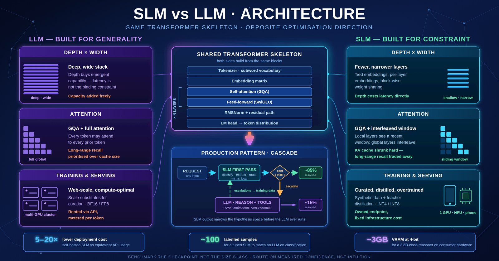
SLM vs LLM, on one page
The whole argument as a single handwritten reference: the shared skeleton, the opposite dials, the 2026 MoE twist, the cascade pattern, and the rules of thumb.
Where the two designs diverge
Both are decoder-only transformers: tokenise, embed, stack attention and feed-forward blocks with residual connections and normalisation, project to a vocabulary distribution. The divergence is in how each layer of that stack is dimensioned and which efficiency techniques are applied.
"Size" stopped being one number
Everything above describes the classical dense picture, and through about 2025 it was the whole story. Two developments have since complicated it enough that the tidy small-versus-large framing needs an amendment.
Mixture-of-experts split size into two independent axes
A sparse MoE model routes each token to a small subset of expert feed-forward blocks, so total parameters and active parameters decouple completely. Gemma 4's 26B-A4B activates roughly 3.8B parameters per token out of 26B total. Qwen 3.5's 35B-A3B routes eight experts plus one shared expert per token for roughly 3B active out of 35B — and claims parity with the previous generation's 235B dense flagship.
The consequence is sharp. Gemma 4's E4B (dense, ~4B) and its 26B-A4B (MoE, ~4B active) have approximately the same inference cost per token and wildly different knowledge capacity. One number no longer describes a model:
| Model | Total params | Active per token | What each number governs |
|---|---|---|---|
| Gemma 4 E2B (dense) | ~5B | ~2B effective | Per-layer embeddings raise effective capacity per stored parameter |
| Gemma 4 E4B (dense) | ~8B | ~4B effective | Same trick, one tier up |
| Gemma 4 26B-A4B (MoE) | 26B | ~3.8B | E4B's compute cost, ~5× the knowledge capacity |
| Qwen 3.5 35B-A3B (MoE) | 35B | ~3B | 8 routed + 1 shared expert per token |
| Phi-4 (dense) | 14B | 14B | Dense — the two numbers are the same |
Active parameters govern latency, throughput and compute cost. Total parameters govern knowledge capacity and memory footprint. A sparse model is cheap to run and expensive to hold — the full weights still have to be resident, which is why the 26B-A4B needs roughly 18GB of VRAM at 4-bit despite behaving like a 4B model at inference time.
The leading edge of small models is no longer purely transformer
The claim that both sides share a transformer skeleton is becoming a simplification. Liquid AI's LFM2.5-2.6B, released in August 2026, stacks 30 layers of which only 8 are grouped-query attention blocks — the other 22 are double-gated short convolution blocks. Attention accounts for roughly 37% of the model. The motive is directly architectural: softmax attention scales quadratically with sequence length, and convolution blocks do not, so replacing most of the attention layers is the cleanest way to buy long context on hardware that has none to spare.
The result is a 2.69B-parameter model with a 131K context window that fits in under 2.5GB and decodes at roughly 220 tokens/second on an Apple M5 Max, about 113 on a Ryzen CPU, and around 30 on a phone. Its own limitations note is worth as much as its benchmarks: the vendor explicitly does not recommend it for coding-heavy or knowledge-intensive work. That is the ceiling from earlier in this article, stated plainly by the people who built the model.
Context windows have largely converged
One correction to a natural misreading of the attention section: windowed attention does not mean small models can't accept long inputs. Context windows of 128K–256K are now routine at small scale. Gemma 4 interleaves local and global attention blocks at a 4:1 ratio for E2B and 5:1 for the rest — most layers are windowed, but global layers remain in the stack.
The efficiency techniques that make SLMs work
None of these are exotic. Most originated in frontier-model research and were adopted downward, because a technique that saves 15% on a cluster becomes existential when the budget is 4GB of phone RAM.
| Technique | What it does | What it costs you |
|---|---|---|
| Grouped-query attention | Multiple query heads share one key/value head, cutting KV cache size and raising throughput | Small quality cost; now near-universal on both sides |
| Sliding-window attention | Some layers attend only to a recent window instead of the full sequence. Gemma 2 interleaved local windows on odd layers with global attention on even ones | Reduced long-range recall on the windowed layers |
| Tied embeddings | Input and output embedding matrices share weights, removing a large parameter block | Minor; standard practice at small scale |
| Per-layer embeddings | Raises effective capacity per stored parameter — how Gemma 4's E2B/E4B variants get "effective" counts below their raw size | More complex runtime, vendor-specific tooling |
| KV cache sharing | Reuses the same cached state across multiple decoder layers. Apple's on-device model does this | Constrains what each layer can specialise in |
| Mixture-of-experts routing | A router activates a few expert FFNs per token, decoupling total from active parameters — Gemma 4's 26B-A4B activates ~3.8B of 26B | Full weights stay resident in memory; routing instability and load imbalance |
| Hybrid conv + attention | Replaces most attention layers with gated short convolutions to escape quadratic scaling — LFM2.5 runs 22 conv blocks to 8 GQA layers | Departs from the pure transformer; younger tooling and less settled theory |
| Latent attention (LLM side) | Compresses keys and values into a low-rank latent space, shrinking the KV cache at frontier scale | More complex to implement; mostly a large-model technique |
| Knowledge distillation | A small student learns from a larger teacher's output distribution rather than hard labels. Used for Gemma 2's 2B and 9B variants | Student inherits teacher's blind spots; needs teacher access |
| Quantisation | Weights dropped from 16-bit to 8-, 4-, or 2-bit. Q4_K_M is the common sweet spot at roughly 4× memory reduction while retaining most benchmark capability | Quality degrades non-uniformly; verify on your task |
Notice that these are not exclusively small-model techniques. Cohere's Command A — an enterprise-scale model — interleaves sliding-window and full attention at a 3:1 ratio, uses GQA and SwiGLU, and applies rotary embeddings on the windowed layers with none on the full-attention ones. The toolkit is shared. What differs is how hard each dial gets turned.
Data quality is the real small-model breakthrough
If architecture were the whole story, small models would still be badly outclassed. The larger shift has been in training recipe, and it rests on three techniques that reinforce each other.
Curation and synthesis. Carefully filtered and deliberately generated training data substitutes for raw volume. Microsoft's Phi line is the clearest demonstration — the thesis is explicitly that data quality can beat raw scale, and Phi-4 at 14B reaching roughly 84.8% MMLU while fitting on a 12GB GPU is the evidence usually cited for it.
Distillation. Most modern SLMs are not trained from scratch; they are descendants of much larger models, learning to imitate a teacher's behaviour and reasoning patterns rather than rediscovering them from a corpus.
Deliberate overtraining. Compute-optimal scaling laws tell you how to spend a fixed training budget for the best model. But if your real constraint is inference cost, the optimum shifts — you train a smaller model on far more tokens than compute-optimal ratios suggest, spending more once to save every time the model runs.
What each one is genuinely good at
LLM — the generalist
Wins where the task is open-ended, the input is unpredictable, or success requires connecting facts across domains the model was never explicitly trained on. Multi-step planning, cross-system root-cause analysis, ambiguous instructions, novel situations, long-context synthesis. Also wins on time-to-first-value: no training data, no fine-tuning, no serving infrastructure.
SLM — the specialist
Wins where the task is well-defined, high-volume, and repetitive — classification, extraction, routing, summarisation of predictable documents, structured formatting. Also wins wherever the constraint is non-negotiable: data cannot leave the building, the device is offline, latency must be single-digit milliseconds, or per-request cost must be effectively zero.
The published evidence supports a sharper claim than most teams expect. On binary classification, small models land within about two points of large ones in zero-shot settings. Fine-tuned specialists need on the order of a hundred labelled examples to match or beat general LLMs across a range of classification tasks. And GLiNER, a purpose-built 50M-parameter model, outperforms general chat models across twenty public named-entity-recognition benchmarks — a model roughly three orders of magnitude smaller winning decisively on a narrow task.
The gap reappears exactly where you would predict. On competitive programming, Phi-4 at 14B reached a pass@3 of around 63.6% against roughly 86.8% for a frontier reasoning model — a gap of some 23 points. Small models also degrade noticeably as prompt complexity rises; they are markedly better suited to simple, well-scoped instructions than to sprawling multi-part ones.
Task-by-task, who should own it
| Workload | Better fit | Reasoning |
|---|---|---|
| Intent / ticket classification | SLM | Stable label set, huge volume, ~100 samples closes the gap |
| Named-entity extraction | SLM | Purpose-built small models beat general models outright here |
| PII redaction before an API call | SLM | Must run locally by definition — that is the whole point |
| Summarising predictable documents | SLM | Small models produce more concise summaries at comparable quality |
| Structured output / schema filling | SLM | Constrained decoding does most of the work |
| Cross-system root-cause analysis | LLM | Requires correlation across domains and genuine novelty |
| Multi-step agent planning | LLM | Plan quality determines step count; weak plans cost more than they save |
| Open-ended code generation | LLM | The measured gap is largest exactly here |
| Ambiguous customer conversations | LLM | Unbounded input distribution, high cost of being wrong |
| Long-context synthesis across sources | LLM | Windowed attention trades away the long-range recall you need |
What people are actually deploying in 2026
The open small-model field has consolidated around a handful of families, each with a distinct centre of gravity. Note the third column of the classification: dense, sparse, or hybrid is now as load-bearing as parameter count. Versions move very fast — Qwen shipped two generations in the months this was written — so treat this as a map of categories rather than a leaderboard.
Some concrete anchors across the size range. At the very bottom, LFM2.5-2.6B fits under 2.5GB and runs agentic tool-calling loops on a phone at around 30 tokens/second — and on a Raspberry Pi 5 at roughly 42. Phi-4-mini at 3.8B occupies about 3GB of VRAM at Q4 and handles modality through LoRA adapters over a frozen base, its speech adapter alone around 460M parameters. Gemma 4's 26B-A4B fits in roughly 18GB at 4-bit while delivering close to the quality of the dense 31B. And Gemma 4 31B reportedly lands within about 10 Elo of open-weight models five to thirty times its size on public leaderboards — the clearest single indicator of how far the efficiency frontier has moved.
On the deployment side, Ollama, llama.cpp, and vLLM handle quantisation without requiring ML expertise, and Qualcomm ships runtimes that execute INT4/INT8 models directly on Snapdragon NPUs. The infrastructure barrier that made self-hosting a specialist team's job three years ago has largely dissolved.
The production answer is almost always a cascade
Framing this as a choice is the mistake. Mature systems run both, with a cheap model handling the volume and an expensive one handling the exceptions. The routing signal can be as simple as a confidence threshold.
Two details make this pattern work better than it looks. First, the SLM's output becomes context for the LLM rather than being discarded — the expensive model starts from a narrowed hypothesis space. Second, every escalation is a labelled training example. Log them, and the SLM's coverage grows over time without anyone running a labelling project.
Three deployments, three different answers
Retail edge inference — SLM, no contest
Retail chains are running 3B-class models on in-store edge servers specifically so that basic functionality survives a network outage. Manufacturing edge AI deployment roughly tripled between 2025 and 2026, with small models as the primary driver. The requirement here isn't "cheaper" — it is that the store must keep working when the link drops. No API can satisfy that, at any price.
Incident root-cause analysis — LLM, no contest
An API latency alert whose actual cause is a config change two tiers upstream in a different cloud requires correlating change records, dependency graphs, and logs across systems that share no schema. The input distribution is unbounded and each incident is novel in its specifics. This is precisely the workload small models degrade on as prompt complexity rises — and precisely what frontier reasoning is for.
Document processing pipeline — hybrid, staged
A realistic split: a local SLM does OCR cleanup, PII redaction, and document-type classification; a mid-size model extracts structured fields against a schema; a frontier LLM handles only the documents that fail validation or arrive in an unrecognised format. Redaction must be local for compliance, extraction is high-volume and schema-bound, and the exception path is genuinely open-ended. Each stage gets the model its constraints actually demand.
Where teams get this wrong
- ▲Choosing on benchmark rank alone. Aggregate scores tell you little about your task. A model that trails on MMLU may win decisively on your ticket taxonomy. Build a small evaluation set from your own data before choosing anything.
- ▲Ignoring the total cost of ownership. A self-hosted SLM is cheap per request and not cheap in aggregate — GPU capacity, quantisation validation, version upgrades, evaluation maintenance, and on-call all land on your team. Below a certain volume the API is genuinely cheaper.
- ▲Assuming quantisation is free. 4-bit retains most capability on most benchmarks, but degradation is uneven and can concentrate in exactly the reasoning or multilingual behaviour you depend on. Re-run your evaluation set post-quantisation, every time.
- ▲Sending complex prompts to small models. They are demonstrably better on simple, well-scoped instructions. If your prompt has six conditional branches, either decompose it or escalate — do not expect the model to absorb the complexity.
- ▲Fine-tuning before trying retrieval or prompting. The cheapest intervention that closes the measured gap wins. Fine-tuning adds a permanent maintenance burden that teams consistently underestimate.
- ▲Underestimating prompt-format sensitivity. Small instruct models can be strict about their expected chat and function-calling templates; deviating from them degrades instruction adherence in ways that look like model weakness but are really integration bugs.
A three-phase evaluation
Two design regions, one toolkit
Small models are extraordinarily capable for their size, and they have a real ceiling — on generalisation, on multi-step reasoning, and on breadth of world knowledge. Both halves of that sentence are true simultaneously, and the engineering skill is in knowing which half applies to the workload in front of you.
Gartner's projection that organisations will use task-specific small models roughly three times more than general large ones by 2027 is not a prediction that large models lose. It is a prediction about workload distribution: most production AI work is repetitive, well-scoped, and high-volume, and that is the shape small models were designed to fill. The hard, novel, unbounded remainder is what frontier models are for — and that remainder is where the value concentrates, not where the volume does.
Design for both. Route between them on measured confidence rather than intuition. And benchmark the specific checkpoint against your own data, because in a field where a 3B model can beat last year's 30B, the size on the label has stopped telling you what you need to know.